
How we made the JVM 40x faster
Java / Scala or any other Java Virtual Machine (JVM) language possesses all the benefits provided by the JVM, but at the same time lacks access to low-level instruction sets required to achieve highest performance. One important example is the intrinsics interface that exposes instructions of SIMD (Single Instruction Multiple Data) vector ISAs (Instruction Set Architectures).
In many cases the JVM is capable of performing some level of vectorization. But this means that SIMD optimizations,
if available at all, are left to the VM and
the built-in just-in-time (JIT) compiler to carry out automatically, which often leads to suboptimal code.
As a result, developers may be pushed to use low-level languages such as C/C++ to gain access to the intrinsics API.
But leaving the high-level ecosystem of Java or other languages also means to abandon many high-level abstractions
that are key for the productive and efficient development of large-scale applications,
including access to a large set of libraries.
To reap the benefits of both high-level and low-level languages, we decided to develop a systematic approach to automatically bring access to low-level SIMD vector instructions to Scala, providing support for all 5912 Intel SIMD intrinsics from MMX to AVX-512. To achieve this we use Lightweight Modular Staging Framework (LMS) and employ a metaprogramming approach to generate and load code in the runtime of the JVM to achieve high performance. Our work builds on top of the LMS Intrinics library that contains support for variety of SIMD eDSLs. Both LMS Intrinics and the JVM runtime extensions have been sumbitted and published at CGO’18, obtaining all 4 badges of the conference: Artifacts Available, Artifacts Functional, Results Replicated and Artifacts Reusable.


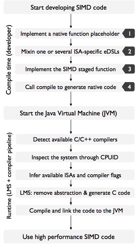
Our approach does not modify the JVM and works on a standard HotSpot JVM. In fact all our tests are performed
on a HotSpot 64-Bit Server 25.144-b01, supporting Java 1.8. An overview of how our system is able to generate fast and
high performance code in the JVM, is given in the figure below depicted in 4 steps:
Let’s illustrate this with a code snippet. Assume we want to implement AVX code that does Level 1 BLAS routine called
SAXPY. This means that we add two vectors x and y into y such that x is scaled by a scalar s. Or in other words y = y + sx.
import ch.ethz.acl.commons.cir.IntrinsicsIR
import com.github.dwickern.macros.NameOf._

class NSaxpy {
  // Step 1: Placeholder for the SAXPY native function
  @native def apply (a: Array[Float], b: Array[Float], scalar: Float, n: Int): Unit
  // Step 2: DSL instance of the intrinsics
  val cIR = new IntrinsicsIR; import cIR._
  // Step 3: Staged SAXPY function using AVX + FMA
  def saxpy_staged(
    a_imm: Rep[Array[Float]], b: Rep[Array[Float]], scalar: Rep[Float], n: Rep[Int]
  ): Rep[Unit] = { import ImplicitLift._
    // make array `a` mutable
    val a_sym = a_imm.asInstanceOf[Sym[Array[Float]]]
    val a = reflectMutableSym(a_sym)
    // start with the computation
    val n0 = (n >> 3) << 3
    val vec_s = _mm256_set1_ps(scalar)
    forloop(0, n0, fresh[Int], 8, (i : Rep[Int]) => {
      val vec_a = _mm256_loadu_ps(a, i)
      val vec_b = _mm256_loadu_ps(b, i)
      val res = _mm256_fmadd_ps(vec_b, vec_s, vec_a)
      _mm256_storeu_ps(a, res, i)
    })
    forloop(n0, n, fresh[Int], 1, (i : Rep[Int]) => {
      a(i) = a(i) + b(i) * scalar
    })
  }

  // Step 4: generate the saxpy function,
  // compile it and link it to the JVM
  compile(saxpy_staged _, this, nameOf(apply _))
}
After the four steps are completed, and the JVM program is started, the compiler pipeline is invoked with the
compile routine. This will perform system inspection, search for available compilers and opportunistically pick
the optimal compiler available on the system. In particular, it will attempt to find icc, gcc or llvm/clang.
After a compiler is found, the runtime will determine the target CPU, as well as the underlying micro-architecture
to derive available ISAs. This allows us to have full control over the system, as well as to be able to pick the
best mix of compiler flags for each compiler.
Once this process is completed, the user-defined staged function is executed, which assembles a computation graph
of SIMD instructions. From this computation graph, LMS generates vectorized C code. This code is then automatically
compiled as a dynamic library with the set of derived compiler flags, and linked back into the JVM.
We then decided to compate our implementation with a standard Java implementation:
public class JSaxpy {
  public void apply(float[] a, float[] b, float s, int n){
    for (int i = 0; i < n; i += 1)
    	a[i] += b[i] * s;
  }
}
Then we benchmarked the code with ScalaMeter. We perform the tests on a Haswell
enabled processor Intel Xeon CPU E3-1285L v3 3.10GHz with 32GB of RAM, running Debian GNU/Linux 8 (jessie),
kernel 3.16.43-2+deb8u3. To obtain precise results, we selected
a pre-configured benchmark that forks a new JVM virtual machine and performs measurements inside the clean instance.
The new instance has a compilation threshold of 100 (-XX:CompileThreshold=100) and we perform at least 100 warm-up
runs on all test cases to trigger the JIT compiler. Each test case is performed on a warm cache. Tests are repeated
30 times, and the median of the runtime is taken. We show the results as performance, measured in flops per cycle.
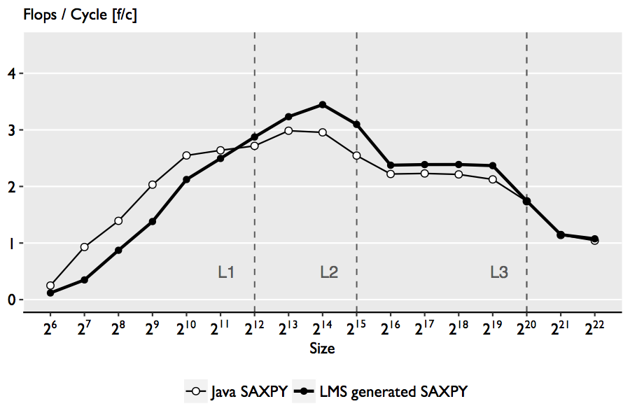
The figure above shows the performance comparison. First we note the similarity in performance, which is not surprising
since SAXPY has low operational intensity and the simplicity of the code enables efficient autovectorization.
To inspect the JIT compilation, we used -XX:UnlockDiagnosticVMOptions that unlocks the diagnostic
JVM options and -XX:CompileCommand=print to output the generated assembly. In all test cases we observe the full-tiered
compilation starting from the C1 compiler to the last phase of the C2 compiler. Then we extract the loop of the
JSaxpy code:
0x00007f0dc07064f0: vmovdqu 0x10(%rcx,%r9,4),%xmm2
0x00007f0dc07064f7: vmulps %xmm1,%xmm2,%xmm2
0x00007f0dc07064fb: vaddps 0x10(%rdx,%r9,4),%xmm2,%xmm2
0x00007f0dc0706502: vmovdqu %xmm2,0x10(%rdx,%r9,4)
Indeed, the assembly diagnostics confirms that the JVM only uses SSE registers, whereas our staged version uses AVX registers and FMA instructions,
which explains the better performance for larger sizes.
Matrix-Matrix-Multiplication Benchmark
While the SAXPY is great for it’s simplicity and assembly analysis, the real performance gain of using SIMD intrinsics
can be shown by tackling compute bound problems. The classical problem being the Matrix-Matrix-Multiplication. We compare
3 versions. The baseline tripple loop implementation:
public void baseline (float[] a, float[] b, float[] c, int n){
    for (int i = 0; i < n; i += 1) {
        for (int j = 0; j < n; j += 1) {
            float sum = 0.0f;
            for (int k = 0; k < n; k += 1) {
                sum += a[i * n + k] * b[k * n + j];
            }
            c[i * n + j] = sum;
        }
    }
}
Blocked version, in order to improve memory locality:
public void blocked(float[] a, float[] b, float[] c, int n) {
    int BLOCK_SIZE = 8;
    for (int kk = 0; kk < n; kk += BLOCK_SIZE) {
        for (int jj = 0; jj < n; jj += BLOCK_SIZE) {
            for (int i = 0; i < n; i++) {
                for (int j = jj; j < jj + BLOCK_SIZE; ++j) {
                    float sum = c[i * n + j];
                    for (int k = kk; k < kk + BLOCK_SIZE; ++k) {
                        sum += a[i * n + k] * b[k * n + j];
                    }
                    c[i * n + j] = sum;
                }
            }
        }
    }
}
And finally, LMS intrinsics generated versious using AVX:
package ch.ethz.acl.ngen.mmm

import ch.ethz.acl.commons.cir.IntrinsicsIR
import com.github.dwickern.macros.NameOf._

class NMMM { self =>

  @native def blocked (a: Array[Float], b: Array[Float], c: Array[Float], n: Int): Unit

  val cIR = new IntrinsicsIR; import cIR._

  def transpose(row: Seq[Exp[__m256]]): Seq[Exp[__m256]] = { import ImplicitLift._
    val __tt = row.grouped(2).toSeq.flatMap({
      case Seq(a, b) => Seq (_mm256_unpacklo_ps(a, b), _mm256_unpackhi_ps(a, b))
    }).grouped(4).toSeq.flatMap({
      case Seq(a, b, c, d) => Seq(
        _mm256_shuffle_ps(a, c, 68), _mm256_shuffle_ps(a, c, 238),
        _mm256_shuffle_ps(b, d, 68), _mm256_shuffle_ps(b, d, 238)
      )
    })
    val zip = __tt.take(4) zip __tt.drop(4)
    val f = _mm256_permute2f128_ps _
    zip.map({ case (a, b) => f(a, b, 0x20) }) ++ zip.map({ case (a, b) => f(a, b, 0x31) })
  }

  def staged_mmm_blocked (
    a: Rep[Array[Float]], b: Rep[Array[Float]], c_imm: Rep[Array[Float]], n: Rep[Int]
  ): Rep[Unit] = { import ImplicitLift._
    val c_sym = c_imm.asInstanceOf[Sym[Array[Float]]]
    val c = reflectMutableSym(c_sym)

    forloop(0, n, fresh[Int], 8, (kk: Exp[Int]) => {
      forloop(0, n, fresh[Int], 8, (jj: Exp[Int]) => {
        //
        // Retrieve the current block of B and transpose it
        //
        val blockB = transpose((0 to 7).map { i =>
            _mm256_loadu_ps(b, (kk + i) * n + jj)
        })
        //
        // Multiply all the vectors of a of the corresponding
        // block column with the running block and store the
        // result
        //
        loop(n, (i: Exp[Int]) => {
          val rowA  = _mm256_loadu_ps(a, i * n + kk)
          val mulAB = transpose(
            blockB.map(_mm256_mul_ps(rowA, _))
          )
          def f(l: Seq[Exp[__m256]]): Exp[__m256] =
            l.size match {
              case 1 => l.head
              case s =>
                val lhs = f(l.take(s/2))
                val rhs = f(l.drop(s/2))
                _mm256_add_ps(lhs, rhs)
          }
          val rowC = _mm256_loadu_ps(c, i * n + jj)
          val accC = _mm256_add_ps(f(mulAB), rowC)
          _mm256_storeu_ps(c, accC, i * n + jj)
        })
      })
    })
  }

  compile(staged_mmm_blocked _, this, nameOf(blocked _))
}
Our Scala implementation uses the SIMD intrinsics with high level constructs of the Scala language, including pattern matching,
lambdas, Scala collections, closures and others that are not available in low-level C code. Once LMS removes the abstraction overhead,
the MMM function results in a high-performance implementation, as shown in the figure below:
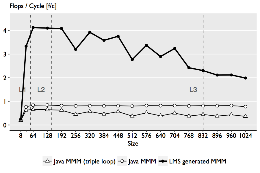
The performance comparison above shows that the use of explicit vectorization through SIMD intrinsics can offer improvements up to 5x over the blocked Java implementation, and over 7.8x over the baseline triple loop implementation.
Machine Learning example: SGD Dot Product
In this benchmark we tackle the building blocks of the SGD algorithm. In particular the dot product operator, performed on two arrays. But instead of standard arrays, we decided to operate on arrays of 32, 16, 8 and 4-bit precision. For 32 and 16-bit we use floating point, which is natively supported by the hardware; for the lower precision formats, we use quantized arrays. Quantization is a lossy compression technique that maps continuous values to a finite set of fixed bit-width numbers. For a given vector of size and precision of bits, we first derive a factor that scales the vector elements into the representable range:
$$ s_v = \frac{2^{b-1} - 1}{\max_{i \in [1, n]} |v_i|}. $$
The scaled are then quantized stochastically:
$$ v_i \rightarrow \left\lfloor v_i \cdot s_v + \mu \right\rfloor $$
where is drawn uniformly from the interval . With this, a quantized array consists of one scaling factor and an array of quantized -bit values.
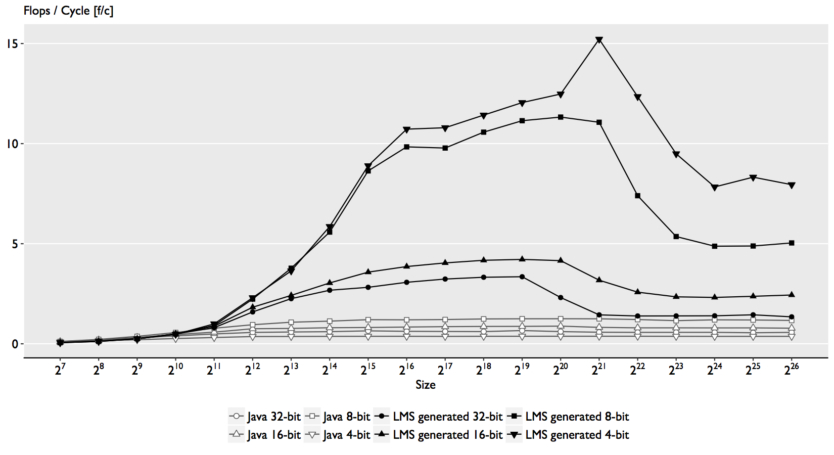
Our 4-bit implementation outperforms HotSpot by a factor of up to 40x, the 8-bit up to 9x, the 16-bit up to 4.8x, and the 32-bit version up to 5.4x.
There are several reasons for the speedups obtained with the use of SIMD intrinsics.
In the 32-bit case, we see the limitation of SLP to detect and optimize reductions.
In the 16-bit, there is no way to obtain access in Java to an ISA such as FP16C.
And in the 8-bit and 4-bit case, Java is severely outperformed since it does type promotion when dealing with integers.
However, the largest speedup of 40x in the 4-bit case is due to the domain knowledge used for the implementing the dot product,
that the HotSpot compiler cannot synthesize with a lightweight autovectorization such as SLP.
To learn more about this work, check out our paper SIMD Intrinsics on Managed Language Runtimes. For in-depth overview of the process of automatic generation of SIMD eDSLs, have a look at the master thesis work of Ivaylo titled Explicit SIMD instructions into JVM using LMS. Also check the code examples and our artefact at https://github.com/astojanov/NGen. Finally, you can also checkout the 20 minute video presentation at CGO which is followed by a short question and answer session.